3D MNIST point cloud classification using Swift for TensorFlow

March 11, 2020 8-minute read

As a passionate Swift developer interested in deep learning, I was intrigued when I first read about Swift for TensorFlow nearly two years ago.

Originating from the TensorFlow team at Google, Swift for TensorFlow (or “S4TF”) is an ambitious open-source project aiming to build a “next generation system for deep learning and differentiable computing”.

Technically speaking, the project itself consists of a branch of the Swift programming language, implementing new compiler features such as first-class differentiable programming support, Python interoperability, static and callable types (landed in Swift 5.2!), and many more.

The “meat” of the project, though, that has motivated these new compiler features can be found in the S4TF deep learning library. Here, you can find the actual Swift package that defines TensorFlow primitives such as optimizers, layers, and operations written entirely in Swift.

For a more complete and well-articulated overview of the project and its goals, see the official “Why Swift for TensorFlow?” post.

3D Convolutional Networks

While S4TF is still very much in active development—and moving quite quickly—I decided to dive in and implement one of the common models that wasn’t yet in the swift-models repo: a 3D convolutional neural network.

Generally speaking, convolutions are filters with learnable parameters that “slide over” input data in order to extract low-dimensional features. Specifically, 3D convolutions are 3-dimensional filters that are useful for extracting features from 3-dimensional input data when we want to preserve the spatial or temporal relationships between our input data.

Here are some example applications of 3D convolutional networks:

Object classification on spatial data (e.g. point clouds)
Medical imagery (e.g. stack of 2D image slices like MRI scans)
Classification of action in video (i.e. UCF-101, UCF-50, HMDB-51)

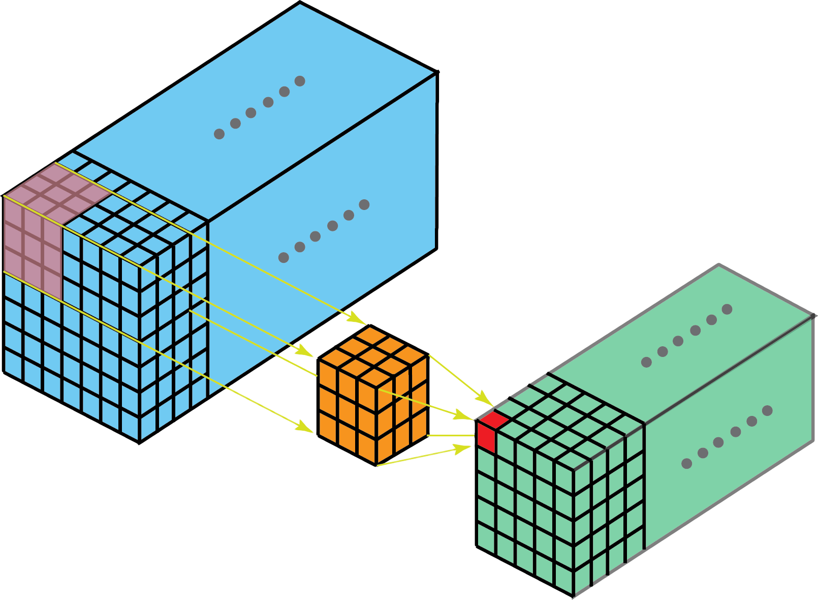
Visualization of 3D convolution over 3 dimensions — towardsdatascience.com

For our network, we’ll choose the domain of object classification and build a digit classifier for 3D MNIST point cloud data.

⚒️ Data Preparation

The 3D MNIST dataset consists of 4096-D vectors obtained from the voxelization (x:16, y:16, z:16) of 3D point clouds. The original dataset contains 10,000 labeled training examples and 2,000 labeled test examples.

💡 Follow along using the completed Colab notebook.

First, after fetching the dataset (full_dataset_vectors.h5), we extract the labels and samples from the HDF5 container and convert them to native S4TF Tensor objects.

let dataset = h5py.File("full_dataset_vectors.h5", "r")

func floatTensor(from data: PythonObject) -> Tensor<Float> {
  return Tensor<Float>(numpy: data.value.astype(np.float32))!
}

func intTensor(from data: PythonObject) -> Tensor<Int32> {
  return Tensor<Int32>(numpy: data.value.astype(np.int32))!
}

var trainingFeatures = floatTensor(from: dataset["X_train"])
var trainingLabels = intTensor(from: dataset["y_train"])

var testFeatures = floatTensor(from: dataset["X_test"])
var testLabels = intTensor(from: dataset["y_test"])

Verify that the shapes of the training and test sets are as expected. Each sample represents an “MNIST digit” in three-dimensional space, where each non-zero element in the 4096-D vector represents a point.

assert(trainingFeatures.shape == TensorShape([10_000, 4096]))
assert(trainingLabels.shape == TensorShape([10_000]))

assert(testFeatures.shape == TensorShape([2_000, 4096]))
assert(testLabels.shape == TensorShape([2_000]))

Next, since we intend to use 3D convolutions, sliding over all three dimensions (x, y, z) of points that comprise each digit, we’ll add an RGB color channel to each sample such that each of the 4096 possible points has a color. The RGB value assigned to each point is simply a mapping of its scalar coordinate into an RGB value based on a specified colormap.

var coloredTrainingSamples = Tensor<Float>(ones: TensorShape([10_000, 4096, 3]))
var coloredTestSamples = Tensor<Float>(ones: TensorShape([2_000, 4096, 3]))

let trainingNp = trainingFeatures.makeNumpyArray()
let testNp = testFeatures.makeNumpyArray()
let scalarMap = cm.ScalarMappable(cmap: "Oranges")

func addColorDimension(scalars: PythonObject) -> Tensor<Float> {
  let rgba = scalarMap.to_rgba(scalars).astype(np.float32)
  let colorValues = Tensor<Float>(numpy: rgba)!
  return colorValues[TensorRange.ellipsis, ..<3] // omit alpha
}

for i in 0 ..< trainingSize {
  coloredTrainingSamples[i] = addColorDimension(scalars: trainingNp[i])
}

for i in 0 ..< testSize {
  coloredTestSamples[i] = addColorDimension(scalars: testNp[i])
}

Finally, the last step in preparing our data is to split the coordinate dimension to three separate dimensions. We use Tensor.reshaped(..) to reshape each sample to be represented as a rank-4 tensor of shape (16, 16, 16, 3).

coloredTrainingSamples = coloredTrainingSamples.reshaped(to: TensorShape(trainingSize, 16, 16, 16, 3))
coloredTestSamples = coloredTestSamples.reshaped(to: TensorShape(testSize, 16, 16, 16, 3))

let coloredTrainingSamplesNp = coloredTrainingSamples.makeNumpyArray()
let trainingLabelsNp = trainingLabels.makeNumpyArray()

print(coloredTrainingSamples.shape) // [10000, 16, 16, 16, 3]
print(coloredTestSamples.shape) // [2000, 16, 16, 16, 3]

📚 Defining the Network

To define our model, we create a Swift struct that conforms to Layer. In it, we make the model callable by implementing callAsFunction(_:) where we specify the transformations to apply to the input data.

Inspiration for this network’s architecture comes from Shashwat Aggarwal’s Keras implementation of 3D-MNIST Image Classification.

let RGB_channels = 3
let classCount = 10

struct Classifier: Layer {
    
    var conv1 = Conv3D<Float>(filterShape: (3, 3, 3, RGB_channels, 8), padding: .same, activation: relu)
    var conv2 = Conv3D<Float>(filterShape: (3, 3, 3, 8, 16), padding: .same, activation: relu)
    var pool = MaxPool3D<Float>(poolSize: (2, 2, 2), strides: (2, 2, 2))

    var conv3 = Conv3D<Float>(filterShape: (3, 3, 3, 16, 32), padding: .same, activation: relu)
    var conv4 = Conv3D<Float>(filterShape: (3, 3, 3, 32, 64), padding: .same, activation: relu)

    var batchNorm = BatchNorm<Float>(featureCount: 64)
    var flatten = Flatten<Float>()
    
    var dense1 = Dense<Float>(inputSize: 4096, outputSize: 4096, activation: relu)
    var dense2 = Dense<Float>(inputSize: 4096, outputSize: 1024, activation: relu)

    var dropout25 = Dropout<Float>(probability: 0.25)
    var dropout50 = Dropout<Float>(probability: 0.5)
  
    var output = Dense<Float>(inputSize: 1024, outputSize: classCount, activation: softmax)

    @differentiable
    func callAsFunction(_ input: Input) -> Output {
      return input
      .sequenced(through: conv1, conv2, pool)
      .sequenced(through: conv3, conv4, batchNorm, pool)
      .sequenced(through: dropout25, flatten, dense1, dropout50)
      .sequenced(through: dense2, dropout50, output)
    }
}

The transformations we choose, defined as Layer subclasses, consist of a series of convolution and pooling (i.e. downsampling) operations ending with a softmax function, which returns a probability distribution of our input point cloud being in each one of 10 possible classes (since there are 10 possible digits). Notice how S4TF defines layers with syntax similar to TensorFlow.

To verify that the model compiles—ensuring there are no inconsistencies with the sizes and shapes of our layers—we create a new Classifier instance and feed in a batch of random data with shape (1, 16, 16, 16, 3).

var model = Classifier()

let dummy = Tensor<Float>(randomNormal: TensorShape(1, 16, 16, 16, 3))
let eval = model(dummy)

assert(eval.shape == TensorShape([1, 10]))

📈 Learning from Data

When it comes to training our model, we group the samples into multiple batches and our model “learns”—that is, updates its internal weights via an optimizer—by iterating over the data in each batch. Batch size is an adjustable hyper-parameter, and for this model we’ll choose a value of 100.

Therefore, for each iteration of the training loop, our model accepts as input a tensor of rank 5 with the following shape: TensorShape(100, 16, 16, 16, 3).

let batchSize = 100
let epochs = 50

let optimizer = Adam(for: model, learningRate: 1e-5, decay: 1e-6)

var trainAccHistory = np.zeros(epochs)
var valAccHistory = np.zeros(epochs)

var trainLossHistory = np.zeros(epochs)
var valLossHistory = np.zeros(epochs)

Also note how we update the learning phase on Context so that the runtime can differentiate between training and inferencing.

for epoch in 0 ..< epochs {

    Context.local.learningPhase = .training

    // Shuffle samples
    let shuffledIndices = np.random.permutation(trainingSize)
    let shuffledSamples = coloredTrainingSamplesNp[shuffledIndices]
    let shuffledLabels = trainingLabelsNp[shuffledIndices]

    // Loop over each batch of samples
    for batchStart in stride(from: 0, to: trainingSize, by: batchSize) {
      let batchRange = batchStart ..< batchStart + batchSize
      let labels = Tensor<Int32>(numpy: shuffledLabels[batchRange])!
      let samples = Tensor<Float>(numpy: shuffledSamples[batchRange])!

      let (_, gradients) = valueWithGradient(at: model) { model -> Tensor<Float> in
          let logits = model(samples)
          return softmaxCrossEntropy(logits: logits, labels: labels)
      }
      optimizer.update(&model, along: gradients)
    }

    // Evaluate model
    Context.local.learningPhase = .inference

    var correctTrainGuessCount = 0
    var totalTrainGuessCount = 0

    for batchStart in stride(from: 0, to: trainingSize, by: batchSize) {
      let batchRange = batchStart ..< batchStart + batchSize
      let labels = Tensor<Int32>(numpy: shuffledLabels[batchRange])!
      let samples = Tensor<Float>(numpy: shuffledSamples[batchRange])!

      let logits = model(samples)

      // accuracy
      let correctPredictions = logits.argmax(squeezingAxis: 1) .== labels
      correctTrainGuessCount += Int(Tensor<Int32>(correctPredictions).sum().scalarized())

      // loss
      trainLossHistory[epoch] += PythonObject(softmaxCrossEntropy(logits: logits, labels: labels).scalarized())
    }

    let trainAcc = Float(correctTrainGuessCount) / Float(trainingSize)
    trainAccHistory[epoch] = PythonObject(trainAcc)

    var correctValGuessCount = 0
    var totalValGuessCount = 0

    for batchStart in stride(from: 0, to: testSize, by: batchSize) {
        let batchRange = batchStart ..< batchStart + batchSize
        let labels = testLabels[batchRange]
        let samples = coloredTestSamples[batchRange]

        let logits = model(samples)

        // accuracy
        let correctPredictions = logits.argmax(squeezingAxis: 1) .== labels
        correctValGuessCount += Int(Tensor<Int32>(correctPredictions).sum().scalarized())

        // loss
        valLossHistory[epoch] += PythonObject(softmaxCrossEntropy(logits: logits, labels: labels).scalarized())
    }

    let valAcc = Float(correctValGuessCount) / Float(testSize)
    valAccHistory[epoch] = PythonObject(valAcc)
    
    print("\(epoch + 1) | Training accuracy: \(trainAcc) | Validation accuracy: \(valAcc)")
}

With this network architecture, we achieve about 68% accuracy on the training set after 50 epochs.

🌐 Unleashing Our Trained Model

With our model fully trained, we can now make inferences to predict the class labels of samples outside the training set!

let randomIndex = Int.random(in: 0 ..< testSize)
var randomSample = coloredTestSamples[randomIndex].reshaped(to: TensorShape(1, 16, 16, 16, 3))

let label = testLabels[randomIndex]

print("Predicted: \(model(randomSample).argmax()), Actual: \(label)")
// Predicted: 9, Actual: 9

📱 From the perspective of an iOS developer, it seems a logical next step would be to export this model to Core ML so that we can classify objects in real-time using our iPhone’s TrueDepth cameras, but unfortunately we can’t (yet!) do so because Conv3D layers aren’t supported by Core ML’s neural network spec. Additionally, at the time of writing, there is not quite yet an official way to export our trained model as a TensorFlow checkpoint.

Note that while we used Colab because of its convenience and built-in Swift for TensorFlow support, there’s no requirement to use it. If, for example, we needed more CPU horsepower or memory for our training process, we could easily spin up our own Jupyter server using the swift-jupyter kernel.

To accompany this post, I’ve submitted a PR to S4TF’s dedicated models repository to add a model similar to the one we’ve built above, a 3D CNN for classifying actions in videos.

💡 Check out the full project code on Colab or GitHub.

Feedback or suggestions? Get in touch with me or contribute to the model on GitHub.

3D Convolutional Networks

⚒️ Data Preparation

📚 Defining the Network

📈 Learning from Data

🌐 Unleashing Our Trained Model

Recommended Resources